Tutorials

This section contains tutorials on how to use the greenWTE package for different applications.

Input Data

As a starting point for any calculating with greenWTE we need to provide the following material properties as input data:

background temperature
velocity operator
phonon frequencies
heat capacities
unit cell volume

Note that the greenWTE cannot treat symmetries at this point, so the full Brillouin zone data is required!

The Material class is used to store these properties. We can create an instance of this class by providing the properties as numpy arrays or using it’s from_phono3py() method to read the data from a phono3py HDF output file. When using the first option all units are assumed to be in SI:

from greenWTE.base import Material

# pass the properties as arrays

material = Material(
    temperature=300,
    velocities=velocities,
    frequencies=frequencies,
    heat_capacities=heat_capacities,
    volume=volume,
)

If data from phono3py is used, the units are automatically converted to SI. Make sure to save the velocity operator when running phono3py and run it with the --nosym flag to get the full Brillouin zone data. The following code snippet shows how to read the data from a phono3py HDF file:

from greenWTE.base import Material

material = Material.from_phono3py("kappa-m191919.hdf5", temperature=300)

For sake of following these tutorials you can use the Silicon and CsPbBr₃ data provided for testing. Note that the 5x5x5 and 4x4x3 q-point meshes used in the tests are not sufficient to obtain converged results! The data can be downloaded by running the tests for the first time and will appear in the test folder. You can create symlinks to the files to be able to easily access them from your working directory with:

ln -sf "$(python -c 'import importlib.resources as r; print(r.files("greenWTE.tests").joinpath("Si-kappa-m555.hdf5"))')" .
ln -sf "$(python -c 'import importlib.resources as r; print(r.files("greenWTE.tests").joinpath("CsPbBr3-kappa-m443.hdf5"))')" .

Static thermal conductivity in bulk

The most basic application of greenWTE is to compute the static thermal conductivity of a bulk material. From here on out we will use the Silicon data provided for testing. First we will use the CLI module solve_iter and then the scripted interface. A full list of the CLI arguments can be found in the CLI Arguments section of the documentation.

Command-line interface

To compute the static thermal conductivity using the CLI we can run the following command in the terminal:

python3 -m greenWTE.solve_iter Si-kappa-m555.hdf5 static_kappa.h5 -k 2.5 -w -300 -t 300 -os none -s gradT

This will compute the thermal conductivity for a spatial frequency of 2.5 rad/m at a temperature of 300 K at a frequency of 1e-300 Hz (i.e. static) using a temperature gradient as the source term, which does not require and outer solver. The results will be saved in the file static_kappa.h5 and the consolue output should look like:

frequency                 κ_xx               κ_xx_P               κ_xx_C     |κ_xx|   |κ_xx_P|   |κ_xx_C|
-----------------------------------------------------------------------------------------------------------
1.00e-300   6.26e+01+4.98e-12j   6.25e+01+4.99e-12j   1.82e-01-1.73e-14j   6.26e+01   6.25e+01   1.82e-01
-----------------------------------------------------------------------------------------------------------

We can see that the total thermal conductivity is only 63 W/m/K, which is far from the experimental value, because of the very coarse q-point mesh. However, the fact that the population contribution is much larger than the coherence contribution is already correctly captured. Let’s see what happens when we do the same thing for CsPbBr₃! Running the following command:

python3 -m greenWTE.solve_iter CsPbBr3-kappa-m443.hdf5 static_kappa.h5 -k 2.5 -w -300 -t 300 -os none -s gradT

we now get a different picture:

frequency                 κ_xx               κ_xx_P               κ_xx_C     |κ_xx|   |κ_xx_P|   |κ_xx_C|
-----------------------------------------------------------------------------------------------------------
1.00e-300   3.13e-01+2.23e-12j   1.03e-01+1.91e-12j   2.10e-01+3.19e-13j   3.13e-01   1.03e-01   2.10e-01
-----------------------------------------------------------------------------------------------------------

The imaginary parts are again very small, but now the coherence contribution is about twice as large as the population contribution! This shows that in materials with strong anharmonicity and complex crystal structures the coherence effects can dominate the thermal transport even at room temperature.

There is a lot more data saved in the output file which is described in save_solver_result().

Scripted interface

To compute the same result using the scripted interface we can use the following code snippet:

from greenWTE.base import Material
from greenWTE.iterative import IterativeWTESolver
from greenWTE.sources import source_term_gradT
from greenWTE.tests.defaults import SI_INPUT_PATH

K_FT = 10 ** 2.5  # spatial frequency in rad/m
material = Material.from_phono3py(SI_INPUT_PATH, temperature=300)
source = source_term_gradT(
    K_FT,
    material.velocity_operator,
    material.phonon_freq,
    material.linewidth,
    material.heat_capacity,
    material.volume,
)
solver = IterativeWTESolver(
    [0],  # static case
    K_FT,
    material,
    source,
    source_type="gradient",
    outer_solver="none",
)
solver.run()

print(f"{solver.kappa[0]:.1f}, {solver.kappa_p[0]:.1f}, {solver.kappa_c[0]:.1f}")

And as expected we get the same result of 63 W/m/K:

62.6...0.0j, 62.5...0.0j, 0.2...0.0j

Try it with the example data for CsPbBr₃ provided and see how the coherence contribution dominates the thermal conductivity in this material at 300K!

Dynamical thermal conductivity in bulk

When using iterative solver we will stick to the scripted interface from now on, but the CLI can be used in the same way. The code snippet from above can be easily adapted to compute the dynamical thermal conductivity by providing an array of temporal frequencies instead of just the static case. To verify the results we can plot the real and imaginary part of the thermal conductivity said frequency range. Assuming you have matplotlib installed, you can run the following code:

from greenWTE import to_cpu, xp
from greenWTE.base import Material
from greenWTE.iterative import IterativeWTESolver
from greenWTE.sources import source_term_gradT
from greenWTE.tests.defaults import SI_INPUT_PATH
import matplotlib.pyplot as plt

K_FT = 10 ** 2.5  # spatial frequency in rad/m
omegas = xp.logspace(7, 14, 20)  # temporal frequencies in rad/s
material = Material.from_phono3py(SI_INPUT_PATH, temperature=300)
source = source_term_gradT(
    K_FT,
    material.velocity_operator,
    material.phonon_freq,
    material.linewidth,
    material.heat_capacity,
    material.volume,
)
solver = IterativeWTESolver(
    omegas,
    K_FT,
    material,
    source,
    source_type="gradient",
    outer_solver="none",
    print_progress=True,
)
solver.run()

f, ax = plt.subplots()

ax.set_xlim(to_cpu(omegas[0]), to_cpu(omegas[-1]))
ax.plot(to_cpu(omegas), to_cpu(xp.real(solver.kappa_p)), "o-", label="$\Re(\kappa_\mathrm{P})$", mec="k")
ax.plot(to_cpu(omegas), to_cpu(xp.imag(solver.kappa_p)), "o-", label="$\Im(\kappa_\mathrm{P})$", mec="k")
ax.set_xscale("log")
ax.set_yscale("log")
ax.set_xlabel("temporal frequency [rad/s]")
ax.set_ylabel("thermal conductivity [W/mK]")
ax.legend()

f.tight_layout()
# plt.show()

(Source code, png)

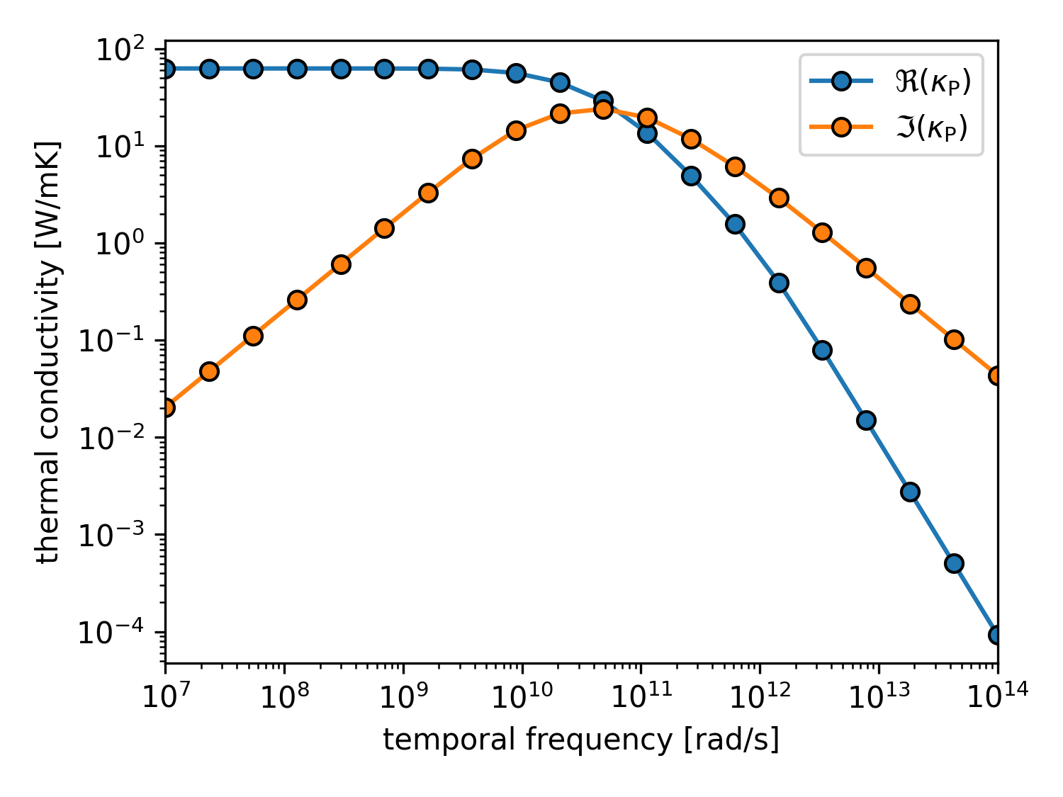
_images/tutorials-1.png — Real and imaginary part of the dynamical thermal conductivity of Silicon at 300K

We can see that the real part of the thermal conductivity decreases with increasing frequency, while the imaginary part first increases and then decreases again. The phase lag between the heat flux and the applied temperature gradient is captured by the imaginary part of the thermal conductivity. Try this for CsPbBr₃ as well and see how the population contributions are suppressed even more strongly at higher frequencies compared to the coherence contributions!

Explicit Green’s-function workflow (save + reuse)

The implicit tutorials above solve the WTE by applying the Wigner operator \(\mathcal{L}\) inside an iterative linear solver. An alternative is to explicitly build and invert \(\mathcal{L}\) once to obtain the Green operator \(\mathcal{G} = \mathcal{L}^{-1}\). This explicit workflow is especially useful when you want to reuse the Green operator for multiple source terms.

The pieces from greenWTE we need are:

RTAWignerOperator assembles \(\mathcal{L}(q;\omega,k)\) (RTA approximation)
RTAGreenOperator inverts it to obtain \(\mathcal{G}(q;\omega,k)\)
GreenContainer stores Green blocks in an HDF5 container on disk
DiskGreenOperator lazily loads the stored Green block so the solver can use it
GreenWTESolver applies \(\mathcal{G}\) to the source term (no inner iterative solve)

Example: compute, save, reload, solve

The script below reproduces the static Silicon example, but explicitly constructs the Green operator, saves it to disk, reloads it, and then solves the WTE using the disk-backed Green operator.

import os
import tempfile

from greenWTE import xp
from greenWTE.base import Material
from greenWTE.green import (
    GreenWTESolver,
    RTAGreenOperator,
    RTAWignerOperator,
    DiskGreenOperator,
)
from greenWTE.io import GreenContainer
from greenWTE.sources import source_term_gradT
from greenWTE.tests.defaults import SI_INPUT_PATH

K_FT = 10 ** 2.5  # spatial frequency in rad/m
omegas = xp.array([0.0])  # static case

material = Material.from_phono3py(SI_INPUT_PATH, temperature=300)
source = source_term_gradT(
    K_FT,
    material.velocity_operator,
    material.phonon_freq,
    material.linewidth,
    material.heat_capacity,
    material.volume,
)

wigner = RTAWignerOperator(omg_ft=float(omegas[0]), k_ft=K_FT, material=material)
green = RTAGreenOperator(wigner)
green.compute()

with tempfile.TemporaryDirectory() as tmp:
    green_path = os.path.join(tmp, "Si-green-T300.hdf5")

    # Save Green's function to disk
    with GreenContainer(
        path=green_path,
        nat3=material.nat3,
        nq=material.nq,
        meta={"temperature": 300},
    ) as gc:
        gc.put_bz_block(omegas[0], K_FT, data=green)

    # Load Green's function from disk
    green_container = GreenContainer(path=green_path, read_only=True)
    green_disk = DiskGreenOperator(
        green_container,
        omg_ft=float(omegas[0]),
        k_ft=K_FT,
        material=material,
    )

    # Solve WTE using the loaded Green's function
    solver = GreenWTESolver(
        omegas,
        K_FT,
        material=material,
        greens=[green_disk],
        source=source,
        source_type="gradient",
        outer_solver="none",
    )
    solver.run()

    print(f"{solver.kappa[0]:.1f}, {solver.kappa_p[0]:.1f}, {solver.kappa_c[0]:.1f}")

And voila, we get the same result as before:

62.6...0.0j, 62.5...0.0j, 0.2...0.0j

This functionality is also exposed in the CLI via precompute_green and solve_green, which are documented in the CLI Arguments section.

This short tutorial should give you a good starting point to use the greenWTE package for your own calculations. Note that the grid for the dataset is not converged, but will give the right trends for many applications. An idea of more sophisticated applications of greenWTE is given in the arXiv preprint “Transition from Population to Coherence-dominated Non-diffusive Thermal Transport” [arXiv:2512.13616 (2025)]. The calculations fully rely on scripts similar to the ones shown in these tutorials.